The objective of this presentation is to explain hypothesis and the aim of hypothesis testing. The hypothesis is the backbone of any research. Hypothesis is important as it emphasize
on researcher's ability to presume the solution. The job of the researcher is to put forward questions with its proposed answers.
The elaborate research process is eleven step process, where researcher deals with hypothesis twice. Basic hypothesis or supposition should be prepared after literature survey. The extensive study of the area of concern helps researcher identify the gaps, all the important factors to be studied and their relationships. All these acts as ingredients for the statement of hypothesis. This hypothesis is tested using statistical measures on data collected.
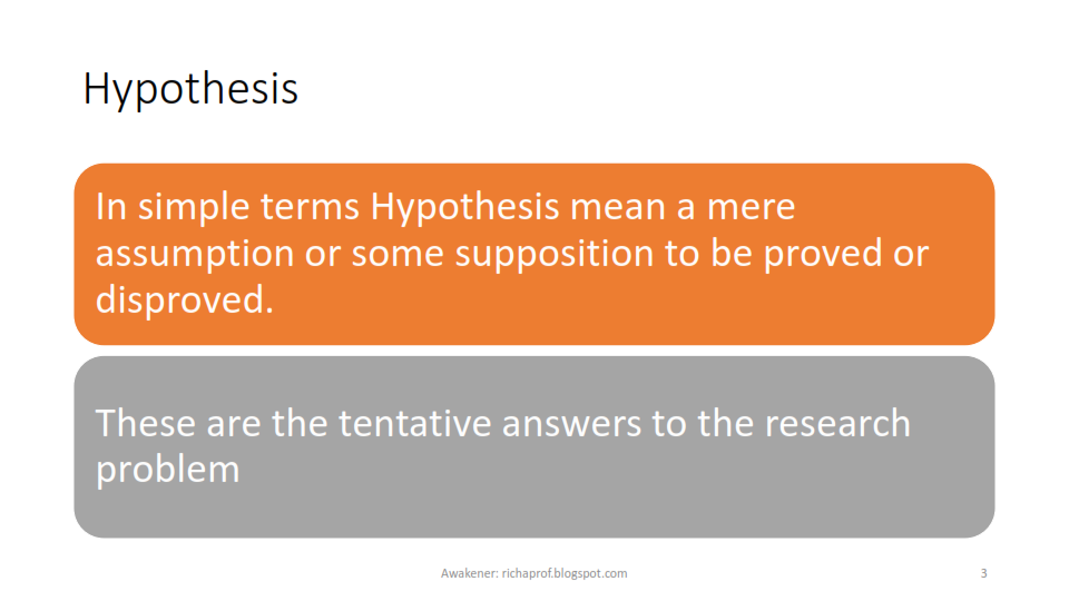
Hypothesis is the intuition of the researcher in terms of what are the probable solutions of the problem in hand. It should contain one dependent variable (criterion) and at least one independent variable (predictor). The aim of the hypothesis testing is to see the relationship between the two i.e. whether the predictor variable actually predicting about the criterion variable or not. Usually they are referred to as predictor and criterion variable in non experimental researches and independent and dependent variable only in experimental research.
In these examples, the hypothesis is stated in the form relationship. In the first example, attendance is the predictor variable, predicting marks of students. In the second example, performance is the predictor variable in judging two brands of automobile.
Hypothesis testing is the process that starts as early as in the step 3 of the process, with the statement of hypothesis and continuous till the penultimate step of the research process.
The Null Hypothesis is the statement of no difference. To begin with, researcher needs to assume that things shall not change because of something or anything. In typical marketing context, any effort (advertising, sales promotion, quality improvement, etc) taken to boost sales will not result in any increase in sales. In other words predictor variable has no control over criterion variable. Medicines will not sustain diseases, performances will not improve, are few examples of null hypothesis.
In some other cases, null hypothesis may state that all the predictor variable (if they are more than one) have equal response or no response to criterion variable. For example, all the factors like price, quality, availability, design, promotion are equally responsible for the success of a brand.
Alternate Hypothesis is the statement other than null. It highlights the differences, effects, and anomalies in the research area. It aims at proving anomalies, not stating the reason behind them though. The aim of the research is prove alternate hypothesis and reject null. For a given null hypothesis there can be many alternate hypothesis.
In a given set observation, the parameters to represent a variable (criterion or predictor) are mean (
X̅) and standard deviation (
σ). In hypothesis testing the means of a sample (X̅) can be tested against the standard mean (µ) or two different samples can be studied ( µ1 and µ2)
The test of difference or no difference would have been be identified by merely looking at means values, but according to the concept of the deviation from mean more precisely, standard deviation (σ), the difference may be because of the extreme values in the observation set. Hence, it is important to see whether the difference in mean values is significant or it is because of the standard deviation. So, the difference is considered as no difference up to a level of significant difference. Since we are checking the probable answer in testing of hypothesis, the level of significance, denoted as α, is taken in terms of percentage probability. Usually, it is set at 5%, which means there is 5% probability that the researcher may state the difference when it is not significant.
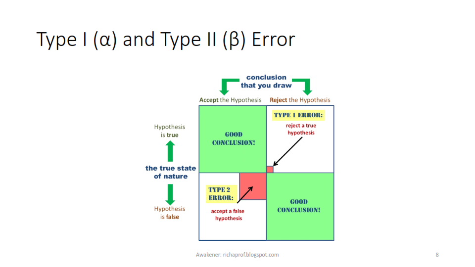
This initiates the discussion on errors in hypothesis testing. Type I error or α-error is committed, when the researcher rejects a null hypothesis when it was true. That means good product is rejected. Type II error or β- error is caused when a null hypothesis is accepted when it was false. That mean accepting a bad product. Type I error is caused due to wrong selection of α. Researcher should have a reasonable level of significance, so that good samples are not rejected. But, in case if the researcher try to increase α he may accept bad samples also and may commit β- error.
It is evident that both types of errors can't be reduced simultaneously. There is trade-off between two -types of error which means probability of making one type of error can only be reduced if the researcher is willing to increase the probability of making the other type of error.The appropriate level of α is decided examining the costs and penalties associated. If the task is to examine engine failures in aircraft it is advisable to keep a low α, but if they are paper planes, high α can be kept. In pharma industry, though, high α is recommended.
There are number of statistical tests available for testing of hypothesis. Depending upon the number of variables used one can select
z-test,
t-test,
χ2 test,
F-test and so on.
Identification of the critical or rejection region using
z-test taking
α = 0.05 based on the central limit theorem that states that in a distribution all the values are equally distributed around the mean or in other words, they follow normal distribution.
Normal distribution is represented by bell shaped curve, at the middle of which the mean is located. According to null hypothesis, the hypothesized
value, say X̅, is equal to the standard value i.e. µ. This is the state of no difference. If the value of X̅ is greater than µ, the z-value moves on the positive (right hand) side and if it is less, z-value moves on negative (left hand) side (see formula for z). Up to some point this more or less is not significant. But as per previously decided value of α , after some z-value the state of difference (more or less) becomes significant.
The total area of normal curve is 1 (i.e. 100% probability). From the symmetry of normal curve, the area (probability) on each side is 0.50.
Two-tailed Test
When the researcher is only trying to identify the difference and not concerned about more or less, the level of significance is equally divided in both sides (tail) of the normal curve.This type of test is called as Two-tailed test. To determine the critical region, 0.025 (i.e.0.05/2) is subtracted from each side and the acceptance region remains to be 0.475 (i.e. 0.50 - 0.025) on each side.

This value when located in z-table, gives z value equals to 1.96
Again, from the property of normal curve z= -1.96 on left hand side and z=1.96 on the right hand side. hence for two-tailed test the acceptance region is between -1.96 to +1.96. For any value of z less than -1.96 or more than +1.96 null hypothesis will be rejected.
One-tailed Test
For identifying more or less situation, the whole 0.05 level of significance is allocated on one side of the normal curve.
For the situation when the researcher wants to reject only the values that are less than standard value. Everything on the right hand side will be accepted and treated as no difference. For example, for testing the hypothesis if the overall performance of an institute has degraded or not, researcher is not interested in the parameters where it is improved, but only look for the parameters where there is a shortfall and aims at checking whether these shortfalls are significant or not.
0.05 will be deducted from left side. the z value will be located for the area 0.45 (i.e. 0.50 - 0.05).
z-table does not have a value equals to 0.45. The two values that are equi-distant from 0.45 are 0.4495 and 0.4505. The
z-value for 0.45 is taken as 1.645, the mean of the respective
z-value of 0.4495 (i.e. 1.64) and 0.4505 (i.e.1.65). Hence the acceptance region is for anything more than -1.645 and the null hypothesis is rejected for any value of
z less than -1.645.
On the other side of the tail, the researcher will only reject if the value is more than some standard value. Here everything on the left hand side is accepted as no difference and the rejection region will lie only on the right tail. For example, if a company wants to know whether the sales of a product is increased or not, it shall only see the higher sales figures for the significant increase.
Here, the null hypothesis is rejected if z value is more than 1.645 and accepted otherwise.
Hopefully, you have now a better understanding of hypothesis and testing of hypothesis. Later, I shall also discuss the alternate method of testing a hypothesis based on
p value.
 This file has two sheets. First has the form responses directly imported from google docs and second sheet is the file ready for coding (after deleting columns like timestamp, name of the respondent, etc).
 Add a new sheet and name it as variables. In the B Column of the Variables sheet right click, paste special. Check Transpose.
 Define all the variables.
 Now, copy the variables and paste its transpose in the sheet1.